Feb 20, 2014 | Uncategorized
Thursday night, I talked about the Baby Boomers and the impact they were having on government spending and the economy. Federal entitlement programs represent a large portion of the U.S Federal budget, and when you combine these programs with the interest on the debt, there isn’t much left over to run the country. As a matter of fact, there isn’t anything left over, and that’s why we need to borrow money every month just to keep the government running (and pay for things like Social Security, Medicare and Medicaid).
So during the Class, I polled the 61 students and asked them to raise their hand if they wanted to reduce Social Security. Nobody raised their hand.
Then I asked if anyone was in favor of reducing Medicare. Same thing, nobody raised a hand.
Finally, after talking about the enormous debt that we were creating with all these programs and the problems they were creating for the economy, I asked if anyone was in favor of reducing Medicare. Again, nobody raised their hand. Not one person in the Class was in favor of reducing or stopping any of these entitlement programs.
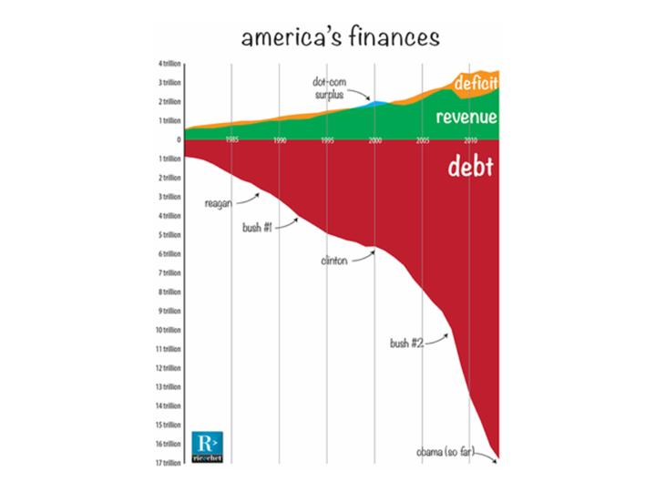
After the discussion, I showed them a chart (attached) of the current debt and how it has continued to grow over the years. I pointed out how the debt has grown independent of who was president. It grew because the majority of people in America want their entitlements.
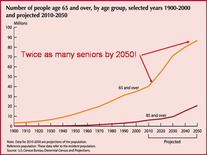
I then showed my students another chart (also attached) that depicts how the number of seniors will continue to grow in the next 25 years, adding to the debt.
After discussing the problems this enormous debt was creating for the economy and the job market, we talked about how the debt could be reduced or paid off.

I asked if anyone was in favor of increasing taxes. Not one hand went up. I asked if anyone would vote for a politician who wanted to raise taxes. Again, not one hand was raised. Hmmm?
So it appears that everybody wants to keep receiving the benefits, but really doesn’t want to pay for them.
Because of this, huge Federal deficits and increasing debt will likely continue in the future. So you need to ask yourself about interest rates. Will they be going up or down? You really don’t need Janet Yellen to tell you this. All you need to do is think about the interest payments on the current debt. They MUST stay low, not for the next few months, or years, but for the foreseeable future…and beyond. If interest rates start to rise, and people want to keep their entitlements, the government will have to borrow even more money, requiring even more interest to be paid to foreigners. The debt is so big now; it will likely NEVER be paid off.
So now you can understand why the Fed MUST do everything in its power to keep interest rates low. It’s not a question of stimulating the economy anymore; it’s a matter of survival!
OK, so how do we deal with this? Well, IF we know that interest rates will likely stay low in the future, we should focus on investments that should do well in a low interest environment.
Several come to mind, like utilities and the banks.
Utilities borrow a lot of money to keep their plants running and expand their facilities to meet the needs of a growing population. They are extremely interest rate sensitive.
I haven’t talked about the utes much on these pages, mainly because almost all of the Fed’s stimulus money was going into other sectors driving the Dow Industrials and NASDAQ technology stocks higher. But this could start to change in the months ahead.
As the Dow moves beyond 16,000, investors, especially seniors, are becoming more risk adverse. Most are only in the market now because they are being forced into it by the government’s low interest rate policy. They can’t live on the interest they receive from CDs or Money Market funds.
But now that the overall market is starting to look overbought and the utilities are near their lows, they are becoming more and more attractive.
Near the end of last year, I started to talk about Consolidated Edison, ED, my favorite Christmas stock. The ‘trade’ didn’t work out this year as ED turned negative after a small pop in mid-November. The stock was in a downtrend when we first looked at it, and wasn’t ready to move higher.
But now, a clear TLB pattern has formed and the PT indicators have turned Green once again. I’m ready to give it another shot. So I will be buying a few shares of ED on Tuesday as a ‘trade’. These shares will go into my IRA account. Remember, ED is still in a down trend, so I can’t fall in love with it. But IF the PT indicators stay Green and it ‘Jumps the Ropes’, I’ll start to add additional shares.
Finding stocks to take advantage of the low interest environment will be the focus of my Big Picture Strategy for 2014. And contrary to popular belief, not all stocks will be able to do this. I’ll discuss why in the days ahead, but it mostly has to do with jobs and the economy.
Fed day pay day
Talking about the Fed. I’m teaching a very special hour long seminar on March 13. 2014 and I’d like to see you there. During this seminar you’ll learn how to cash in on fed day and get two BONUS insights included. It’s perfect for exploiting the fed day.
Feb 10, 2014 | Uncategorized
This Traders’ Tip is based on “The Degree Of Complexity” by Oscar Cagigas in the February issue of
Stocks & Commodities.
The five Donchian breakout systems described by Cagigas in his article are coded using the following rules:
| System |
Entry rule |
Exit rule |
Entry price formula |
Exit price formula |
| 2 Param-Long |
Buy2P |
ExitBuy2P |
Buy2Ppr |
ExitBuy2Ppr |
| 2 Param-Short |
Sell2P |
ExitSell2P |
Sell2Ppr |
ExitSell2Ppr |
| 4 Param-Long |
Buy4P |
ExitBuy4P |
Buy4Ppr |
ExitBuy4Ppr |
| 4 Param-Short |
Sell4P |
ExitSell4P |
ell4Ppr |
ExitSell4Ppr |
| 6 Param-Long |
Buy6P |
ExitBuy6P |
Buy6Ppr |
ExitBuy6Ppr |
| 6 Param-Short |
Sell6P |
ExitSell6P |
Sell6Ppr |
ExitSell6Ppr |
| 8 Param-Long |
Buy8P |
ExitBuy8P |
Buy8Ppr |
ExitBuy8Ppr |
| 8 Param-Short |
Sell8P |
ExitSell8P |
Sell8Ppr |
ExitSell8Ppr |
| 9 Param-Long |
Buy9P |
ExitBuy9P |
Buy9Ppr |
ExitBuy9Ppr |
| 9 Param-Short |
Sell9P |
ExitSell9P |
Sell9Ppr |
ExitSell9Ppr |
The EDS code file has the backtests already set up for all of these long and short rules. In Figure 5, I show a typical setup for the pricing. In Figure 6, I show a typical setup for the exit rule.

FIGURE 5: AIQ. Here is a typical setup for the pricing portion of the backtests.
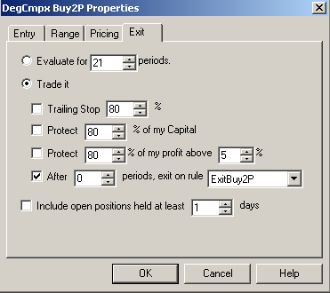
FIGURE 6: AIQ. Here is a typical setup for the exit portion of the backtests.
!THE DEGREE OF COMPLEXITY
!Author: Oscar G. Cagigas, TASC Feb 2014
!Coded by Richard Denning 12/7/13
!www.TradersEdgeSystems.com
! CODING ABBREVIATIONS:
C is [close].
H  is [high].
L  is [low].
O is [open].
PEP  is {position entry price}.
PD     is {position days}.
! PARAMETERS:
donLen1 is 40.
donLen2 is 15.
atrLen is 20.
atrMult is 1.0.
atrStop  is 4.0.
maLen1  is 10.
maLen2  is 100.
rsiLen is 14.
rsiUpper  is 70.
rsiLower  is 30.
atrMult2 is 0.6.
minMov is 0.01.
!------------------------------------------------------------------
! AVERAGE TRUE RANGE (AS DEFINED BY WELLS WILDER)
WWE is 2*(atrLen-1).
TR  is Max(H - L,max(abs(valresult(C,1) - L),abs(valresult(C,1)- H))).
ATR is expAvg(TR,WWE).
ATR1 is valresult(ATR,1).
!------------------------------------------------------------------
!! RSI WILDER
!To convert Wilder Averaging to Exponential Averaging use this formula:
!ExponentialPeriods = 2 * WilderPeriod - 1.
U  is C-valresult(C,1).
D  is valresult(C,1)-C.
eLen is 2 * rsiLen - 1.
AvgU  is ExpAvg(iff(U>0,U,0),eLen).
AvgD  is ExpAvg(iff(D>=0,D,0),eLen).
rsi  is 100-(100/(1+(AvgU/AvgD))).
!----------------------------------------------------------------
!BASIC SYSTEM 2P (2 parameters):
HHdL1 is  highresult(H,donLen1,1).
HHdL2 is  highresult(H,donLen2,1).
LLdL1 is lowresult(L,donLen1,1).
LLdL2 is lowresult(L,donLen2,1).
Buy2P if H > HHdL1.
ExitBuy2P if  L < LLdL2.
Sell2P if L < LLdL1.
ExitSell2P if H > HHdL2.
Buy2Ppr is max(O,HHdL1 + minMov).
ExitBuy2Ppr is iff(ExitBuy2P,min(O,LLdL2 - minMov),C).
Sell2Ppr is min(O,LLdL1 - minMov).
ExitSell2Ppr is max(O,HHdL2 + minMov).
!-----------------------------------------------------------------
!FOUR PARAMETER SYSTEM 4P:
Buy4P if H > HHdL1 and valrule(TR < atrMult*ATR,1).
EB4P1 if L < LLdL2.
EB4Pval is PEP - atrStop*valresult(ATR,PD).
EB4P2 if L < valresult(EB4Pval,1).
ExitBuy4P if EB4P1 or EB4P2.
Sell4P if L < LLdL1 and valrule(TR < atrMult*ATR,1).
ES4Pval is PEP + atrStop*valresult(ATR,PD) .
ES4P1 if H > HHdL2.
ES4P2 if H > valresult(ES4Pval,1).
ExitSell4P if ES4P1 or ES4P2.
Buy4Ppr is max(O,HHdL1 + minMov).
ExitBuy4Ppr is iff(EB4P1,min(O,LLdL2 - minMov),
iff(EB4P2,min(O,valresult(EB4Pval - minMov,1)),-99)).
Sell4Ppr is min(O,LLdL1 - minMov).
ExitSell4Ppr is iff(ES4P1,max(O,HHdL2 + minMov),
iff(ES4P2,max(O,valresult(ES4Pval + minMov,1)),-99)).
!----------------------------------------------------------------
!SIX PARAMETER SYSTEM 6P:
SMA1 is simpleavg(C,maLen1).
SMA2 is simpleavg(C,maLen2).
Buy6P if H > HHdL1 and valrule(TR < atrMult*ATR,1)
and valrule(SMA1 > SMA2,1).
EB6P1 if L < LLdL2.
EB6Pval is PEP - atrStop*valresult(ATR,PD).
EB6P2 if L < valresult(EB6Pval,1).
ExitBuy6P if EB6P1 or EB6P2.
Sell6P if L < LLdL1 and valrule(TR < atrMult*ATR,1)
and valrule(SMA1 < SMA2,1).
ES6Pval is PEP + atrStop*valresult(ATR,PD) .
ES6P1 if H > HHdL2.
ES6P2 if H > valresult(ES6Pval,1).
ExitSell6P if ES6P1 or ES6P2.
Buy6Ppr is max(O,HHdL1 + minMov).
ExitBuy6Ppr is iff(EB6P1,min(O,LLdL2 - minMov),
iff(EB6P2,min(O,valresult(EB6Pval - minMov,1)),-99)).
Sell6Ppr is min(O,LLdL1 - minMov).
ExitSell6Ppr is iff(ES6P1,max(O,HHdL2 + minMov),
iff(ES6P2,max(O,valresult(ES6Pval + minMov,1)),-99)).
!---------------------------------------------------------------
!EIGHT PARAMETER SYSTEM 8P:
Buy8P if H > HHdL1 and valrule(TR < atrMult*ATR,1)
and valrule(SMA1 > SMA2,1) and valrule(RSI >= rsiUpper,1).
EB8P1 if L < LLdL2.
EB8Pval is PEP - atrStop*valresult(ATR,PD).
EB8P2 if L < valresult(EB8Pval,1).
ExitBuy8P if EB8P1 or EB8P2.
Sell8P if L < LLdL1 and valrule(TR < atrMult*ATR,1)
and valrule(SMA1 < SMA2,1) and valrule(RSI <= rsiLower,1).
ES8Pval is PEP + atrStop*valresult(ATR,PD) .
ES8P1 if H > HHdL2.
ES8P2 if H > valresult(ES8Pval,1).
ExitSell8P if ES8P1 or ES8P2.
Buy8Ppr is max(O,HHdL1 + minMov).
ExitBuy8Ppr is iff(EB8P1,min(O,LLdL2 - minMov),
iff(EB8P2,min(O,valresult(EB8Pval - minMov,1)),-99)).
Sell8Ppr is min(O,LLdL1 - minMov).
ExitSell8Ppr is iff(ES8P1,max(O,HHdL2 + minMov),
iff(ES8P2,max(O,valresult(ES8Pval + minMov,1)),-99)).
!----------------------------------------------------------------
!NINE PARAMETER SYSTEM 9P:
Buy9P if H > HHdL1 and valrule(TR < atrMult*ATR,1)
and valrule(SMA1 > SMA2,1) and valrule(RSI >= rsiUpper,1)
and valrule(TR > atrmult2*ATR,1) .
EB9P1 if L < LLdL2.
EB9Pval is PEP - atrStop*valresult(ATR,PD).
EB9P2 if L < valresult(EB9Pval,1).
ExitBuy9P if EB9P1 or EB9P2.
Sell9P if L < LLdL1 and valrule(TR < atrMult*ATR,1)
and valrule(SMA1 < SMA2,1) and valrule(RSI <= rsiLower,1)
and valrule(TR > atrmult2*ATR,1) .
ES9Pval is PEP + atrStop*valresult(ATR,PD) .
ES9P1 if H > HHdL2.
ES9P2 if H > valresult(ES9Pval,1).
ExitSell9P if ES9P1 or ES9P2.
Buy9Ppr is max(O,HHdL1 + minMov).
ExitBuy9Ppr is iff(EB9P1,min(O,LLdL2 - minMov),
iff(EB9P2,min(O,valresult(EB9Pval - minMov,1)),-99)).
Sell9Ppr is min(O,LLdL1 - minMov).
ExitSell9Ppr is iff(ES9P1,max(O,HHdL2 + minMov),
iff(ES9P2,max(O,valresult(ES9Pval + minMov,1)),-99)).
!----------------------------------------------------------------
Feb 3, 2014 | Uncategorized
In my previous article I wrote about a simple “system” – if you can even call it that – that involves buying retailing stocks four months out of the year and holding cash the rest of the year. As ridiculously simple as that sounds the fact of the matter is that if you earned just 1% of annualized interest while out of retailing stocks, the system outperformed a buy-and-hold approach by a fairly wide margin.
While the results of that simple system aren’t bad, as always, one can’t help but to look for ways to improve things. So this article will detail what I refer to as – and by the way, this is what I sound like when I refer to myself in the third person – “Jay’s Energetic Market Shoppers” System, or JEMS (clever, no?) for short. The name is derived from the investment vehicles involved:
1. J stands for, well, OK, Jay….
2. E stands for “Energetic”: Energy stocks have showed a historical tendency to rally in the spring so we will hold Fidelity Select Energy (ticker FSENX) during the month of April (other possibilities include tickers XLE and ENPIX).
3. M stands for “Market”: The stock market tends to perform well during November, December and January. We are already planning to hold retail stocks during November, but for December and January we will hold an S&P 500 index fund. For the purposes of this test we will use the S&P 500 Index itself from 1988 into 1997. From there we will use the ETF ticker SPY. Someone who wanted to keep it all in the Fidelity family could use ticker VFINX. (Another possibility is ticker BLPIX).
4. S is or “Shoppers”: Just as with the original system, we will hold Fidelity Select Sector Retailing (ticker FSRPX) during February, March, October and November (other possibilities include tickers XLY and CYPIX).
During May, June, July, August and September we will hold cash.
So here is the “lineup”
January SPY
February FSRPX
March FSRPX
April FSENX
May Cash
June Cash
July Cash
August Cash
September Cash
October FSRPX
November FSRPX
December SPY
So how does it work out? Not too badly. Figure 1 displays the growth of $1,000 using the JEMS System versus buying and holding the S&P 500.
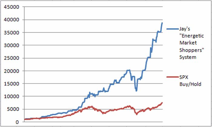 Figure 1 – Growth of $1,000 using “Jay’s Energetic Market Shoppers” System versus buying and holding the S&P 500 since 1988.
Figure 2 displays the year-by-year results.
|
JEMS
|
S&P 500
|
|
JEMS
|
S&P 500
|
|
Annual %
|
Annual %
|
Difference
|
$1,000
|
$1,000
|
|
1988
|
25.4
|
12.4
|
7.0
|
1,254
|
1,124
|
|
1989
|
12.4
|
27.3
|
(27.6)
|
1,410
|
1,430
|
|
1990
|
12.2
|
(6.6)
|
28.7
|
1,582
|
1,336
|
|
1991
|
36.6
|
26.3
|
(9.4)
|
2,161
|
1,688
|
|
1992
|
27.7
|
4.5
|
16.6
|
2,760
|
1,763
|
|
1993
|
10.5
|
7.1
|
(0.1)
|
3,050
|
1,888
|
|
1994
|
10.5
|
(1.5)
|
0.7
|
3,369
|
1,859
|
|
1995
|
8.1
|
34.1
|
(31.1)
|
3,642
|
2,493
|
|
1996
|
19.5
|
20.3
|
(2.1)
|
4,353
|
2,998
|
|
1997
|
14.2
|
31.0
|
(18.4)
|
4,970
|
3,927
|
|
1998
|
50.5
|
26.7
|
14.3
|
7,479
|
4,975
|
|
1999
|
42.4
|
19.5
|
(7.9)
|
10,652
|
5,946
|
|
2000
|
(2.4)
|
(10.1)
|
19.4
|
10,400
|
5,343
|
|
2001
|
15.6
|
(13.0)
|
16.8
|
12,027
|
4,646
|
|
2002
|
3.5
|
(23.4)
|
36.9
|
12,450
|
3,561
|
|
2003
|
10.5
|
26.4
|
(16.6)
|
13,755
|
4,500
|
|
2004
|
18.9
|
9.0
|
4.6
|
16,354
|
4,905
|
|
2005
|
(1.1)
|
3.0
|
6.2
|
16,182
|
5,052
|
|
2006
|
14.8
|
13.6
|
(3.7)
|
18,574
|
5,740
|
|
2007
|
2.4
|
3.5
|
(5.3)
|
19,027
|
5,943
|
|
2008
|
(30.4)
|
(38.5)
|
7.0
|
13,237
|
3,656
|
|
2009
|
33.2
|
23.5
|
1.0
|
17,635
|
4,513
|
|
2010
|
32.5
|
12.8
|
14.0
|
23,366
|
5,090
|
|
2011
|
17.2
|
(0.0)
|
14.0
|
27,381
|
5,090
|
|
2012
|
21.3
|
13.4
|
4.7
|
33,204
|
5,772
|
|
2013
|
16.7
|
29.6
|
(18.2)
|
38,752
|
7,481
|
|
|
|
|
|
|
|
|
Average
|
16.3
|
9.6
|
1.3
|
|
|
|
StdDev
|
16.1
|
17.9
|
|
|
|
|
Ave/SD
|
1.011
|
0.540
|
|
|
|
Figure 2 – Year-by-Year Results
For the record:
-The JEMS System sported an average annual gain of +16.3%
-Buy/Hold sported an average annual gain of +9.6%
-$1,000 invested using the system grew to $38,752
-$1,000 invested using Buy/Hold grew to $7,481
-The JEMS system showed a gain in 23 of 26 calendar years (88.5%)
-The JEMS system showed a loss in 3 of 26 calendar years (12.5%)
-Buy/Hold showed a gain in 19 of 26 calendar years (73.1%)
-Buy/Hold showed a loss in 7 of 26 calendar years (26.9%)
-JEMS outperformed Buy/Hold in 15 of 26 calendar years (57.7%)
-Buy/Hold outperformed JEMS in 11 of 26 calendar years (42.3%)
Summary
So is the JEMS System the “world beater” system that everyone should be using? Well, on the plus side the long-term results are impressive relative to buy and hold. On the downside, there is still the sharp drawdown of 2008 that one would have had to continue to trade through. Also, the reality is that for most investors, a system like this involves more of a “leap of faith” than they are comfortable with.
Of course, as a proud graduate of “The School of Whatever Works” and as a founding member (OK, so far the only member) of “Seasonalaholics Unanimous!”……
………that’s just the way I like it.
Jay Kaeppel
Chief Market Analyst at JayOnTheMarkets.com and AIQ TradingExpert Pro (http://www.aiq.com) client
Jay has published four books on futures, option and stock trading. He was Head Trader for a CTA from 1995 through 2003. As a computer programmer, he co-developed trading software that was voted “Best Option Trading System” six consecutive years by readers of Technical Analysis of Stocks and Commodities magazine. A featured speaker and instructor at live and on-line trading seminars, he has authored over 30 articles in Technical Analysis of Stocks and Commodities magazine, Active Trader magazine, Futures & Options magazine and on-line at www.Investopedia.com.
Jan 28, 2014 | Uncategorized
Hi, my name is Jay and I am a Seasonalaholic.
Now typically when someone confesses to being an “aholic” of some sort or another it because they recognize they have a problem and wish to correct it. That’s not the case here. In fact the “support” group that I belong to is not “Seasonalaholics Anonymous” but rather “Seasonalaholics Unanimous!” (OK, in the interest of full disclosure, so far I am the only member and yes, the monthly meetings aren’t terribly lively, but I digress).
Still I can’t help but think there are others out there who might join someday – especially after they consider things like the seasonal tendencies for retailing stocks. To whit: what would have happened had an investor invested in Fidelity Select Sector Retailing fund (ticker FSRPX):
-During the months of February, March, October and November
-And then earned 1% of annualized interest while out of the market the other 8 months.
The answer is contained in Figure 1 which displays the growth of $1,000 invested as described above.
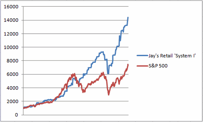 Figure 1 – Growth of $1,000 invested in FSRPX during February, March, October, November (blue line) versus buying and holding the S&P 500 red line) since January 1988.
Now it is pretty impossible to not notice the, ahem, “slight drawdown” experienced during the October, November 2008 period. Still, despite the fact that I have tried very hard scrub that particular time period from my memory bank, I still have some vague recollection that virtually no sector of the stock market was left unscathed during that period. And the rebound has been pretty nice.
So is this really a viable strategy? Well, under the category of “Everything is Relative”, Figure 2 displays the year-by-year performance of this “system” versus buying and holding the SP 500.
|
System |
SP 500 |
|
System |
SP 500 |
|
Annual % |
Annual % |
Difference |
$1,000
|
$1,000
|
|
1988
|
18.6
|
12.4
|
6.2
|
1,186
|
1,124
|
|
1989
|
(1.0)
|
27.3
|
(28.2)
|
1,174
|
1,430
|
|
1990
|
21.3
|
(6.6)
|
27.8
|
1,424
|
1,336
|
|
1991
|
16.2
|
26.3
|
(10.1)
|
1,654
|
1,688
|
|
1992
|
20.4
|
4.5
|
15.9
|
1,992
|
1,763
|
|
1993
|
6.2
|
7.1
|
(0.9)
|
2,115
|
1,888
|
|
1994
|
(1.5)
|
(1.5)
|
0.0
|
2,083
|
1,859
|
|
1995
|
2.3
|
34.1
|
(31.8)
|
2,131
|
2,493
|
|
1996
|
17.4
|
20.3
|
(2.9)
|
2,500
|
2,998
|
|
1997
|
11.9
|
31.0
|
(19.1)
|
2,798
|
3,927
|
|
1998
|
40.1
|
26.7
|
13.4
|
3,919
|
4,975
|
|
1999
|
10.8
|
19.5
|
(8.7)
|
4,344
|
5,946
|
|
2000
|
8.5
|
(10.1)
|
18.7
|
4,714
|
5,343
|
|
2001
|
3.1
|
(13.0)
|
16.1
|
4,859
|
4,646
|
|
2002
|
12.8
|
(23.4)
|
36.2
|
5,480
|
3,561
|
|
2003
|
9.1
|
26.4
|
(17.3)
|
5,977
|
4,500
|
|
2004
|
12.8
|
9.0
|
3.8
|
6,744
|
4,905
|
|
2005
|
8.5
|
3.0
|
5.5
|
7,316
|
5,052
|
|
2006
|
9.2
|
13.6
|
(4.4)
|
7,991
|
5,740
|
|
2007
|
(2.4)
|
3.5
|
(6.0)
|
7,797
|
5,943
|
|
2008
|
(32.0)
|
(38.5)
|
6.5
|
5,303
|
3,656
|
|
2009
|
23.7
|
23.5
|
0.2
|
6,559
|
4,513
|
|
2010
|
26.0
|
12.8
|
13.2
|
8,263
|
5,090
|
|
2011
|
13.2
|
(0.0)
|
13.2
|
9,355
|
5,090
|
|
2012
|
17.3
|
13.4
|
3.9
|
10,976
|
5,772
|
|
2013
|
10.7
|
29.6
|
(18.9)
|
12,155
|
7,481
|
| |
|
|
|
|
|
| Average |
10.9
|
9.6
|
1.3
|
+1,115% |
648% |
| StdDev |
12.8
|
17.9
|
|
|
|
| Ave/SD |
0.849
|
0.540
|
|
|
|
Figure 2 – “System” versus S&P 500 Buy and Hold
Summary
The difference in the average annual return is not large (+10.9% for the system versus +9.6% for the S&P 500). But this difference adds up over time. Since January 1988 the system has gained +1,115% versus + 648% for the S&P 500 (while only being in the market 33% of the time. The true “numbers geeks” will notice that the standard deviation of annual returns for the system is only 2/3rds as large as that for the S&P 500 – i.e., much less volatility).
So I ask again, is this really a viable strategy? Perhaps. But the truth is that it can get a whole lot better – as I will detail the next time I write.
Jay Kaeppel
Chief Market Analyst at JayOnTheMarkets.com and AIQ TradingExpert Pro (http://www.aiq.com) client
Jay has published four books on futures, option and stock trading. He was Head Trader for a CTA from 1995 through 2003. As a computer programmer, he co-developed trading software that was voted “Best Option Trading System” six consecutive years by readers of Technical Analysis of Stocks and Commodities magazine. A featured speaker and instructor at live and on-line trading seminars, he has authored over 30 articles in Technical Analysis of Stocks and Commodities magazine, Active Trader magazine, Futures & Options magazine and on-line at www.Investopedia.com.
Jan 22, 2014 | Uncategorized
To date, Hank Swiencinski aka The Professor, has delivered two sold out premium webinars to traders, his powerful ‘Rifle Trades’ and his widely acclaimed ‘Trading the Turns’.
The demand for these courses exceeded our quota both times, so much so that we had to offer the recording and the seminar book as a product after the events.
The Professor’s next premium event will be on March 13, 2014 and it’s sure to sell out.
So what’s with the title? The Professor, will be presenting another webinar on March 14th that will focus on the techniques he uses to trade the markets on event driven days like the Fed Announcement.
He calls these techniques ‘Going to the Candy Store’. Like all of the techniques in the Professor’s Methodology, they are extremely easy to understand and apply. With the right setup and technical analysis, these special days in the market can be money in the bank. It’s not rocket science, it’s commonsense and simple technique.
This webinar will also include 2 BONUS insights that The Professor uses in his every day trading, including one that predicts moves of 100 points or more, a day or two before the moves actually occur.
SEATS SELL OUT FAST
Jan 21, 2014 | Uncategorized
There are a virtually unlimited number of ways to play the financial markets. This is especially true in the area of options trading, where a bullish trader can pick from at least at a dozen different strategies (buy call, buy a bull call spread, sell a bull put spread, collar, out-of-the-money calendar spread, etc., etc.).
At some point it can all become a bit overwhelming to the quote, unquote, “average investor.” So sometimes the place to start is, well, anywhere, so long as that anywhere has a beginning and an end and a logical progression to it. What does that mean? It means I am going to walk through “one way to play.” I make no claim that it is the “best” way, or even a “great” way. But that’s OK because the purpose here is not for you to rush out and start trading with it, but rather to stimulate your own thinking on the subject. In other words, hopefully in reading this a “light” will go on for you in regards to your own trading. So here goes.
Jay’s “Light” Option Trading Strategy
This strategy involves a set of steps designed to generate a bullish option trade based on a logical set of criteria. For this strategy we will look for a couple of things:
1. A “catalyst” to tell us when to buy call options.
2. Stocks that enjoy good option trading volume and tight bid-ask spread.
3. Stocks that are performing well overall.
4. Stocks that have experienced a recent pullback and may now be due for a bounce.
#1. The “Catalyst”
We will look for ticker SPY to be above its 200-day moving and for the 3-day RSI to drop to 20 or below and then reverse to the upside. Figure 1 displays a number of such signals.
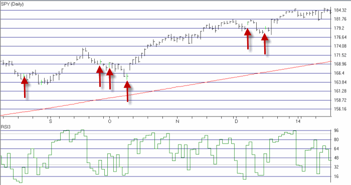 Figure 1 – “Catalyst” Buy Signals (Courtesy AIQ TradingExpert)
#2. Stocks with good option volume and tight bid/ask spreads.
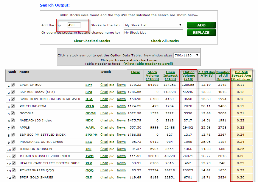
In Figure 2 we see the “Stock List Filter” report from www.OptionsAnalysis.com. This list contains 493 stocks that trade at least 1,000 options a day and those options have an average bid/ask spread of less than 2% (only the top part of the list is visible in Figure 2).
#3. Stocks that are performing well overall
Next we take the stocks shown in Figure 2 and run them through the “Channel Finder” routine in www.OptionsAnalysis.com. We will look for the top 100 stocks based on the strength of their “Up Channel”. We overwrite “My Stock List” with just those 100 stocks. The output list appears in Figure 3.
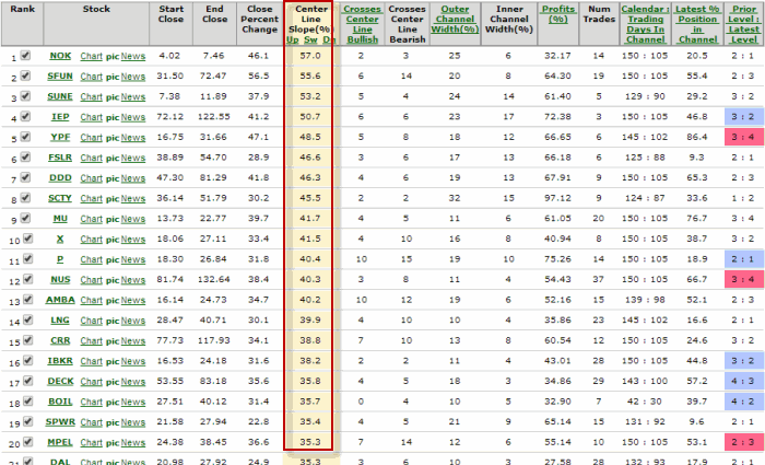
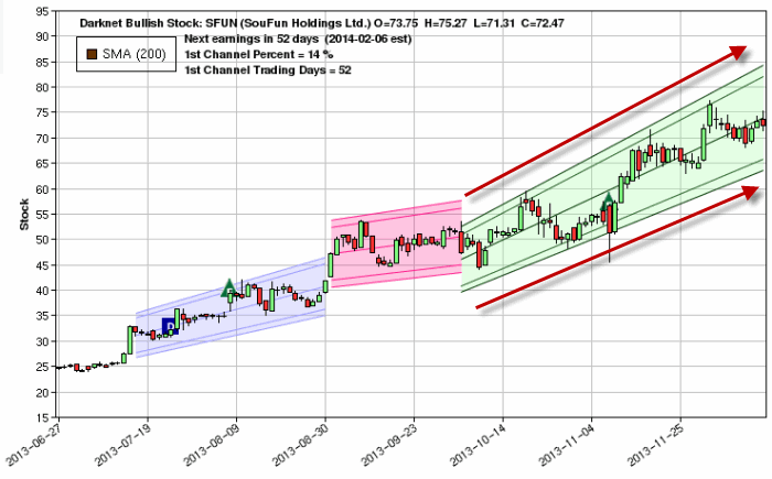
In Figure 4 we see ticker SFUN with a very strong recent Up Channel
#4. Stocks that have experienced a “pullback”
Lastly, we will look through the 100 stocks still on our list for those that have experienced a 3-day RSI of 35 or less within the past 5 trading days. As you can see in Figure 5, only 19 stocks now remain for consideration.
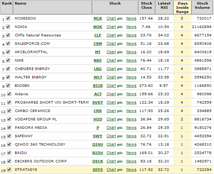 Figure 5 – Stocks that have had a 3-day RSI reading of 35 or less in past 5 days (Courtesy: www.OptionsAnalysis.com)
The Next Step: Finding a Trade
From here a trader can use whatever bullish option strategy they prefer to find a potentially profitable trade among these 19 stocks. For illustrative purposes we will:
-Consider buying calls with 45 to 145 days left until expiration and Open Interest of at least 100 contracts.
-Initially sort the trades by a measure known as “Percent to Double”, as in “what type of percentage move does the underlying stock have to make in order for the option to double in price?”
-Once we get that list e will sort by “Highest Gamma” in an effort to get the most “bang for the buck.”
We see the output list in Figure 6.
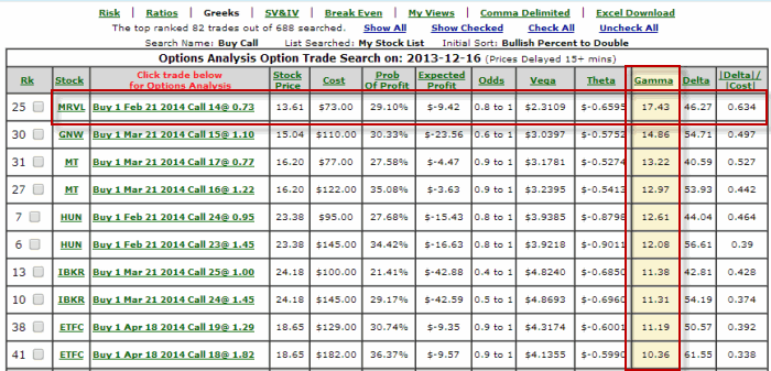
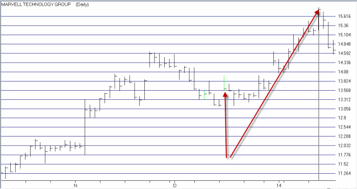
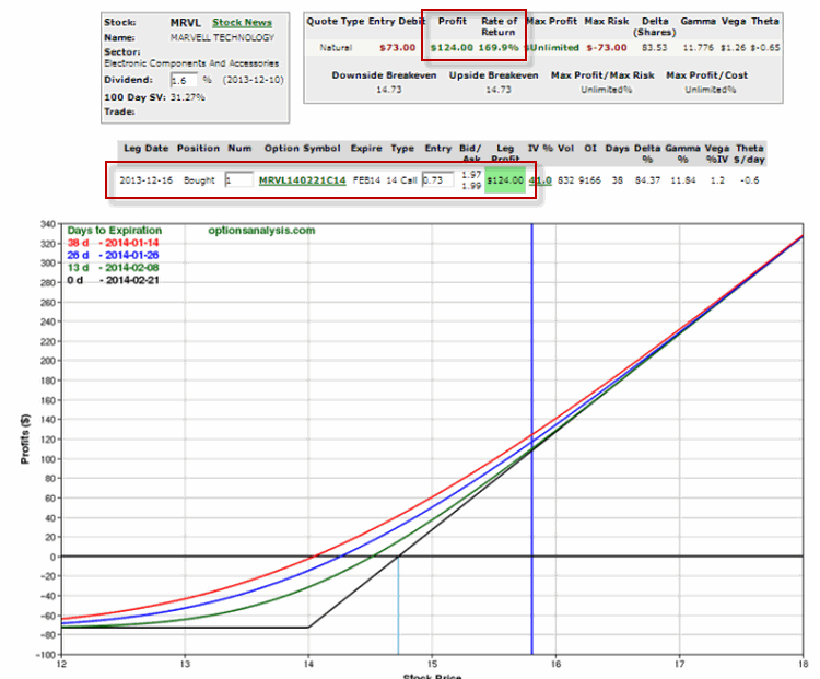
The top trade listed in to buy the MRVL Feb 2014 14 Call @ $0.73 (or $73 per option)
In Figure 7, we see that MRVL rallied nicely within a few weeks from 13.61 to 15.81.
In Figure 8 we see that the Feb 14 call option gained 169.9%.
Of course there is also the whole topic of what to do with this trade: close it, sell some, adjust it, etc. Sorry folks, that’s beyond the scope of this article.
Summary
So does every trade work out this well? That reminds me of a joke. A salesman rings he doorbell of a home and a 12–year old boy answers the door. The boy has a beautiful woman on each side, a drink in one hand and a big cigar in his mouth. Momentarily stunned the salesman finally manages to ask hesitantly, “Um, is your mother home?”
The boy removes the cigar from his mouth, looks straight at the salesman and asks, “What do you think?”
Same answer here. Still, a logical set of steps is a good place to start.
Jay Kaeppel
Chief Market Analyst at JayOnTheMarkets.com and AIQ TradingExpert Pro (http://www.aiq.com) client
Jay has published four books on futures, option and stock trading. He was Head Trader for a CTA from 1995 through 2003. As a computer programmer, he co-developed trading software that was voted “Best Option Trading System” six consecutive years by readers of Technical Analysis of Stocks and Commodities magazine. A featured speaker and instructor at live and on-line trading seminars, he has authored over 30 articles in Technical Analysis of Stocks and Commodities magazine, Active Trader magazine, Futures & Options magazine and on-line at www.Investopedia.com.